Fine-grained topographic organization within somatosensory cortex during resting-state and emotional face-matching task and its association with ASD traits | Translational Psychiatry – Autism Love

The dataset that was used for the current analysis was part of the EU-AIMS LEAP project, a multi-site European collaborative effort with its main aim to identify biomarkers associated with ASD. The study design is described extensively in an earlier publication by Loth et al. [22] along with a comprehensive overview of the clinical characterization of the cohort [23] (for data acquisition details, see Supplementary Material).

Resting-state functional MRI (rfMRI) scans were available for 656 participants, to which we applied a set of stringent quality control exclusion criteria. Participants with a structural brain abnormality (not clinically relevant; n = 17), an incomplete rfMRI scan (n = 8), excessive head motion during the rfMRI scan (mean frame-wise displacement > .7 mm[n = 29; 5% highest average head motion in our sample], max frame-wise displacement> 3.8 mm[n = 38; 1 voxel size]), or insufficient brain coverage (n = 24) were excluded (n = 145). We further excluded participants with insufficient variance of voxels in the selected region of interest and/or poorly estimated connectopies (n = 107; see Section ‘Connectopic Mapping’). This resulted in the inclusion of 404 participants with rfMRI scans.

For the emotional processing task, we used the Hariri emotion processing fMRI task [24] performed by 287 participants. This task followed a block design paradigm and each block included 6 trials of the same task (face or shape). Each of the two runs included 3 face blocks and 3 shape blocks, with 8 s of fixation at the end of each run. The participants were presented with blocks of trials that either ask them to decide which of two faces presented on the bottom of the screen match the face at the top of the screen(experimental condition), or which two shapes presented at the bottom of the screen match the shape at the top of the screen (control condition). The faces have either an angry or fearful expression and each lock is preceded by a 3000 ms task cue, so that each block is 21 s including the cue. After quality control, we included 249 participants in the analysis.

Demographic and clinical characteristics of our sample for rfMRI and the Hariri task can be found in Table 1 and Table 2, respectively.

Table 1 Participant demographic and clinical characteristics for neurotypical (NT) and autistic (ASD) participants with rfMRI.

Full size table

Preprocessing of both the rfMRI and task fMRI was performed using a standard preprocessing pipeline that included tools from the FMRIB Software Library (FSL version 5.0.6; http://www.fmrib.ox.ac.uk/fsl). For the rfMRI data, we initially recombined the three rfMRI scan echoes using echo-time weighted averaging. Preprocessing included removal of the first five volumes to allow for signal equilibration, primary head motion correction via realignment to the middle volume using MCFLIRT [25], global 4D mean intensity normalization and spatial smoothing with a 6 mm FWHM Gaussian kernel. Then, ICA-AROMA was used to identify and remove secondary motion-related artifacts [26, 27]. Next, nuisance regression was applied to remove signal from white matter and CSF, and a 0.01 Hz high-pass filter was applied to remove very low-frequency drifts in the time-series data. To preserve the broad-band characteristics of functional connectivity data no low-pass filtering was applied [28]. The fMRI images of each participant were co-registered to the participants’ high-resolution T1 anatomical images via boundary-based registration (BBR) implemented in FSL FLIRT [25]. The T1 images of each participant were registered to MNI152 standard space with FLIRT 12-dof linear registration [29], and further refined using FNIRT non-linear registration (10 mm warp, 2 mm resampling resolution) [25]. Finally, we brought all participant-level fMRI images to 2 mm MNI152 standard space, in which all further analyses were conducted.

Clinical measures

The autistic participants have received clinical diagnosis according to the DSM-IV, ICD-10, or DSM-5 criteria. Furthermore, additional dimensional measures of sensory processing, social and adaptive functioning for both neurotypical and autistic participants were available. The Short sensory profile (SSP) [30] was used to assess sensory processing atypicalities across 38 items from which an overall raw score was derived that reflects sensory processing across multiple sensory domains. The Repetitive Behaviors Scale-Revised (RBS-R) was used to measure the repetitive behavior observed in individuals. The Social Responsiveness Scale-Second Edition (SRS-2) [31] was used to assess distinctions in social behavior associated with ASD across a 65-item rating scale. The overall T-scores from parent and self-reports (for neurotypical adults, SRS-2 self-report version of the questionnaire was administered, while for the rest a parent-reported symptom questionnaire was available) are reported here. Finally, the Vineland Adaptive Behavior Scales, Second Edition (Vineland-II) [32] a semi-structured parent interview, was used to assess the adaptive functioning of participants across three domains: communication, socialization, and daily living skills. For a more extensive description of all the existing clinical measures of this project, check the work from Charman et al. [23].. The Autism Diagnostic Interview-Revised (ADI-R) and Autism Diagnostic Observation Scale (ADOS-2) were the two diagnostic instruments used in the diagnosis of autistic individuals. The studies reported in the introduction used the aforementioned dimensional measures SRS-2 and Vineland-II to explore the link between sensory atypicalities and difficulties in social life or adaptive functioning, respectively. Additionally, repetitive behaviors, another key feature of ASD, have also been linked with different aspects of sensory atypicalities (e.g., heightened level of tactile seeking) [33].

The differential availability of the measures led to a limited subgroup of participants examined for each one (Table 1 and Table 2). However, repeating the analysis using imputed measures led to similar conclusions. The imputed measures were estimated using Extra Tree multivariate regression, a method that outperformed all other imputation strategies evaluated in the specific dataset (e.g., K-nearest neighbors, Bayesian Ridge Regression, mean and median variable imputation) [34].

Connectopic mapping

We selected the post-central gyrus based on the Harvard–Oxford atlas (available as part of FSL [35]) as our region of interest. Based on this ROI we estimated connection topographies (‘connectopies’) [17] separately for each participant, hemisphere, and imaging measure (rfMRI, Hariri task) using congrads (publicly available at https://github.com/koenhaak/congrads). This analysis approach involves three main steps and is summarized in Fig. 1 of the Supplementary Material. Briefly though, first we obtain the connectivity fingerprint of each somatosensory voxel computed as the Pearson correlation between the voxel-wise time series from the predefined ROI and the losslessly SVD-transformed time series from all gray-matter voxels outside the ROI. We then insert the fingerprint matrix to a manifold learning algorithm (Laplacian eigenmaps) to obtain a set of connection topographies. The derived connectopies represent how the connectivity between the target ROI and the rest of the cortex varies topographically within the specified ROI. Finally, we fit a spatial statistical model (a ‘trend surface model’) to each connection topography. In this work, we focus on the first and primary connectopy derived from this method, which closely follows the somatotopic organization. The position along the colorbar of the connectopy reflects the similarity between the connectivity profile with similar colors indicating similar functional connectivity profile.

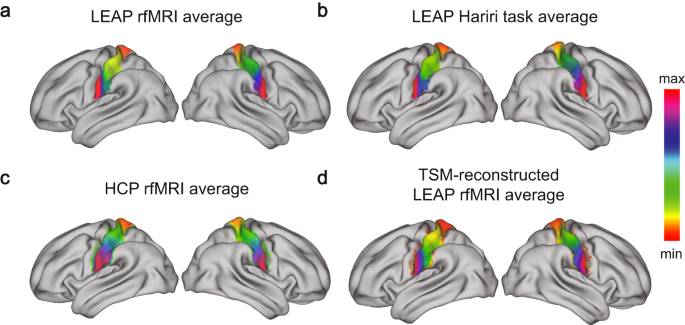
**Fig. 1: Somatosensory connectopies in LEAP and HCP datasets.**

Illustration for both hemispheres of the a average S1 connectopy at rest in the LEAP dataset, the b average S1 connectopy during the Hariri task in the LEAP dataset, the c HCP S1 connectopy, used as a reference, and the d TSM-reconstructed (6^th model order) average S1 connectopy at rest in the LEAP dataset. The colorbar indicates the position along the primary mode of connectivity change – similar colors represent similar connectivity patterns.

Trend Surface Modelling (TSM) was applied to the connectopies to obtain a lower-dimensional representation which facilitates further statistical inference [17]. By applying TSM to our connectopies, we obtain a set of parameters (‘TSM coefficients’) that correspond to polynomial coefficients of varying order along 3D Euclidian axes and summarize the connectopies as a set of spatial polynomial basis functions. The polynomial degree, i.e., the number of TSM coefficients, controls the granularity of the representation of the connectopic map and was chosen based on the value that minimized the model’s Bayesian information criterion (BIC) while, at the same time, maximizing its explained variance (EV).

We further used a reference connectopy derived from the well-known excellent quality rfMRI dataset Human Connectome Project (HCP) in which the somatotopic organization of the primary motor cortex has been mapped before [17]. We compared the connectopies between the two datasets, so that we get an estimation of the quality of the obtained LEAP connectopies, as well as of the validity of the main axis of connectivity change that we observe. To sensitize our analyses to subtle variations within connectopies, while ensuring that poor-quality connectopies do not unnecessarily inflate the polynomial degree, individuals whose connectopies correlated less than r = 0.5 with the reference HCP connectopy were excluded from further analysis (n = 99 [neurotypical:autistic=54:45]; see ‘Data preparation for connectopic mapping’ in Supplementary Material).

Additionally, we estimated the projection maps of the connectopies onto the rest of the brain by using dual regression to map the whole-brain connectivity changes associated with the subtle variations within the ROI [36]. Dual regression allows us to obtain subject-wise spatial maps based on group-ICA components, avoiding the pitfall of comparing components that are not well-matched between subjects, but rather derive from differences in decomposition across them.

Association with clinical measures and comparison between connectopies

The Pearson’s correlation coefficient between the TSM coefficients of the connectopies and the available clinical measures was calculated. We additionally controlled for biological sex, age, full-scale IQ and site via OLS multiple regression. Separate GLM analysis on raw connectopies was conducted using as explanatory variables ASD diagnosis, sex, age, and the clinical and behavioral scores reported in Table 1, as a complementary analysis to ensure the polynomial fitting of the connectopies does not limit our results. P-values have been corrected for multiple comparisons via the Bonferroni-Holm method (FWER = 0.05). We compared the connectopies between groups of neurotypical and autistic individuals, as well as between rest and task, using t-tests, independent and paired samples, respectively. The spatial correlation between connectopies was calculated in a voxel-wise manner. The implementation code is publicly available at https://github.com/cisakoglou/congrads_sensory_leap.

Average connectopies estimated across individuals during rest and the Hariri task

For the modeling of the S1 connectopy the 6^th order was selected for our model (see Supplementary Fig. 2). This entailed the representation of each connectopy with a set of 18 parameters (x, y, z, x², y², z², x³, etc.) during both rest and task. That is, spatial variation within the ROI was modeled through a trend surface that was described by polynomials up to 6^th order in x,y, and z direction.

The average connectopy across all individuals – autistic and neurotypical individuals combined – is illustrated in Fig. 1a for rest and Fig. 1b for task. After visual inspection, we observe the similarity with the average connectopy estimated from HCP (Fig. 1c). The voxel-wise spatial correlation between the HCP connectopy and the one during each imaging measure (task and rest) was estimated (HCP-rest: (left hemisphere) Pearson’s r = 0.83, (right hemisphere) Pearson’s r = 0.94; HCP-task: (left hemisphere) Pearson’s r = 0.89, (right hemisphere) Pearson’s r = 0.96; p-values < .001 for all four comparisons).

The average S1 connectopy along the dorsoventral axis of each hemisphere was reproduced across both conditions and datasets with similar reconstructions of the connectopies for all (see reconstruction for the average S1 connectopy during rest in Fig. 1d) and matches the somatotopic organization.

Association between S1 connectopies and ASD dimensional measures

During the Hariri task, a significant correlation was found between two TSM coefficients (z², z⁴) reconstructing the S1 connectopy of the left hemisphere and Vineland-II Daily Living scores (see Supplementary Material). Correlations with the Vineland-II Socialization and Adaptive Behavior Composite (ABC) standard scores were also high but did not survive multiple comparisons correction. The complete results of the correlation analysis during the Hariri task can be found in Supplementary Figs. 4 and 5. We performed a sensitivity analysis to ensure those results are not driven by edge effects by repeating the analysis on the eroded connectopies of 50 randomly selected participants and the TSM coefficients were not found to differ significantly between the original and the eroded connectopies (see Supplementary Fig. 14). This resulted in almost identical associations with the behavioral scores as well.

We conducted a separate GLM analysis on raw S1 connectopies to examine the localization of the above correlation and ensure that the observed effects are not driven by limitations from the polynomial modeling. As reported in Supplementary Figs. 8–10, Vineland-II Daily-Living, Socialization and Communication scores survived correction, and the association was mostly located at the S1/M1 boundaries.

During rest, some TSM coefficients (see Supplementary Material) were found to be correlated with Vineland-II Daily Living and Vineland-II ABC scores. However, these correlations did not withstand multiple comparisons correction. We also correlated TSM coefficients with SSP, SRS-2, and Vineland-II Socialization, and no significant relationship was found. The complete results of the correlation analysis during rest can be found in Supplementary Figs. 6 and 7.

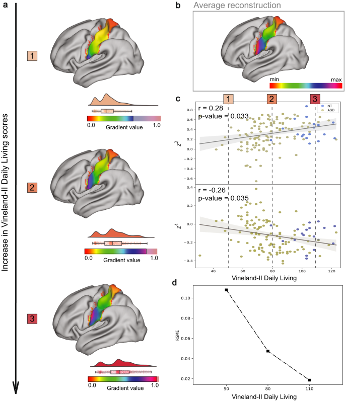
In addition, we aimed to understand how the S1 connectopy during the Hariri task changes as a function of variation within clinical measures. Having already obtained the TSM coefficients reconstructing the S1 connectopy and the respective clinical measure with which they were associated, we visualized the clinical associations of the underlying topography in the following manner; We derived TSM-reconstructed connectopies at three evenly spread points across the Vineland-II Daily Living scale (Fig. 2a) by fitting their original reconstructions to the average TSM-reconstructed connectopy (Fig. 2b) and obtaining their respective residual connectopies. The points across the Vineland scale that were selected are highlighted as 1,2 and 3 in Fig. 2c.

**Fig. 2: Visualization of the change in the connectivity profile within left hemisphere’s S1 during the Hariri task as a function of the Vineland-II Daily Living scores.**

In a we visualize the reconstructions of the connectopies that correspond to the three evenly spread selected points across the Vineland-II Daily Living scale highlighted in (c). The arrow indicates the direction towards which the Vineland-II Daily Living scores increase – reflecting higher functioning. The gradients’ color range varies along this increase in the functioning scale which is illustrated by a raincloud visualization shifting its max value more towards the extreme of the color range in each of the reconstructions. We further illustrate in b the TSM-reconstructed average S1 connectopy of the left hemisphere during the Hariri task, in c the scatterplots of the two TSM coefficients z² and z⁴ reconstructing the S1 connectopies and which were found to be significantly associated with Vineland-II Daily Living scores, and in d the Root Mean Square Error (RMSE) between the reconstructed S1 connectopy of each of the three aforementioned selected points from Vineland-II Daily Living scale and the average S1 reconstructed connectopy. The decrease of RSME observed with the increase of the Vineland-II Daily Living scores demonstrates how similar the S1 connectopy gets with the average one as the individuals’ functioning gets higher.

We further calculated the root-mean-square error (RMSE) between the TSM coefficients reconstructing the average connectopy in the z direction – this includes the coefficients that were found to correlate significantly with Vineland-II scores – and the TSM coefficients reconstructing the connectopy and corresponding to each of the selected points on the Vineland-II Daily Living scale highlighted in Fig. 2c. In Fig. 2c, we have shown how the RMSE decreases as a function of the adaptive Vineland-II scores (see also the reconstruction of average connectopy for neurotypical individuals only in Supplementary Fig. 11). This provides an estimation of the reduction in flatness observed within the S1 connectopy as functioning skills improve.

We have shown that as adaptive functioning increases, expressed by higher Vineland-II Daily Living scores, the color range within the gradient of the reconstructed connectopy becomes wider, reflecting a broader ROI to rest-of-brain differential connectivity pattern. Conversely, the gradient becomes flatter toward the other end of the Vineland scale, indicating lower functioning skills. The S1 connectopy of individuals with higher functioning skills, encompassing the broader range of differential connectivity, and the high model order that captures the more subtle changes of the connectopy, suggest higher functional differentiation in these individuals. Lower functional differentiation, on the other hand, is associated with lower adaptive ability, but this does not indicate the absence of a specific S1 function.

Comparison between the connectopies of neurotypical and autistic individuals

Group comparisons of the S1 connectopies between neurotypical and autistic individuals did not yield any significant results for either hemisphere for both imaging measures (task and rest; see Supplementary Fig. 3). During the Hariri task, there were three TSM coefficients (y², y⁴, and y⁶ [p-values: 0.017, 0.019, 0.025] for the left hemisphere) that were nominally significant but did not survive multiple comparisons correction (see Supplementary Material for visualization of the group comparison).

Connectopic similarities and differences during rest and task

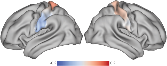
To elucidate further the nature of the established association between connectopies and adaptive scores, we examined in more detail the differences between intrinsic functional connectivity (iFC) gradients during rest and task connectopies. Despite the dorsoventral axis of the connectopy being reproduced in both rest and task, we observed significant differences between the two. The TSM coefficients that were found to differ in the 192 participants for whom the scans of both conditions were available were 6 coefficients on the z-axis for the left hemisphere and 5 coefficients on the x- and y-axis for the right one (see Supplementary Material). The disparities between the rest and task connectopies are displayed in Fig. 3, highlighting a global, rather than a focal, pattern of differences along the dorsoventral axis of the S1.

**Fig. 3: Differences between rfMRI and Hariri task S1 connectopies.**

Visualization of the connectopic differences after averaging the differences between the individual S1 connectopies during rfMRI and Hariri task (Connectopy_rfMRI – Connectopy_Hariri).

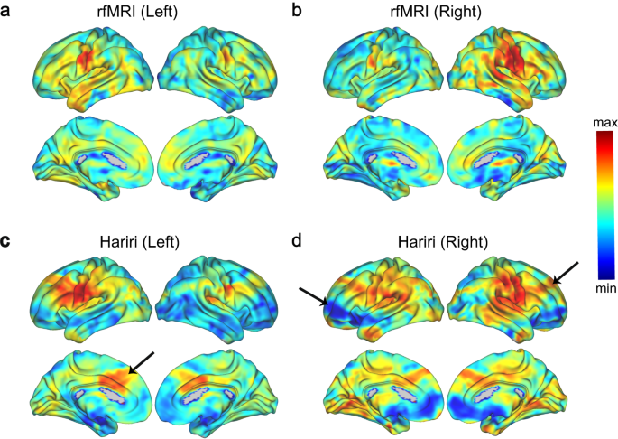
We additionally estimated the projections of the S1 connectopies onto the brain to highlight further the spatial components involved in the connectivity profile changes we observe. Projections during rest from the left and right hemisphere’s S1 connectopy are illustrated respectively in Fig. 4a, b and for the Hariri task in Fig. 4c, d. Overall, the color-gradients present in the left/right hemisphere reappear contralaterally in the opposite hemisphere, providing evidence that the two sensory strips are topographically connected. There is a general convergence between the two imaging measures (task and rest) (projections(left): Pearson’s r = 0.85 [p-value < .001], projections(right): Pearson’s r = 0.77 [p-value < .001]), apart from a frontal component – including frontal gyrus and anterior cingulate gyrus extending to the insular cortex (see Supplementary Figs. 12 and 13) – that seem to have enhanced similarity in its connectivity profile with S1 during task and a prefrontal component, on the opposing end, with a highlighted lack of similarity during task, more evident for the right hemisphere.

Projection maps of the S1 connectopies onto the entire brain during the rfMRI from the left and right hemisphere in (a) and (b) respectively, and during the Hariri task from the left and right hemisphere in (c) and (d) respectively. The arrows highlight the regions with connectivity profile of enhanced or diminished similarity with the S1 connectopy during task. These regions correspond respectively for the enhanced and diminished similarity cases to the anterior cingulate gyrus and frontal gyrus, and to a prefrontal component of the right hemisphere.

This content was originally published here.